Understanding Optimizers in Machine Learning

If you remember anything from Calculus (not a trivial feat), it might have something to do with optimization. Finding the best numerical solution to a given problem is an important part of many branches in mathematics, and Machine Learning is no exception. Optimizers, combined with their cousin the Loss Function, are the key pieces that enable Machine Learning to work for your data.
This post will walk you through the optimization process in Machine Learning, how loss functions fit into the equation (no pun intended), and some popular approaches. We’ll also include some resources for further reading and experimentation.
What is an Optimizer in Machine Learning?
We’ve previously dealt with the loss function, which is a mathematical way of measuring how wrong your predictions are.
During the training process, we tweak and change the parameters (weights) of our model to try and minimize that loss function, and make our predictions as correct and optimized as possible. But how exactly do you do that? How do you change the parameters of your model, by how much, and when?
This is where optimizers come in. They tie together the loss function and model parameters by updating the model in response to the output of the loss function. In simpler terms, optimizers shape and mold your model into its most accurate possible form by futzing with the weights. The loss function is the guide to the terrain, telling the optimizer when it’s moving in the right or wrong direction.
For a useful mental model, you can think of a hiker trying to get down a mountain with a blindfold on. It’s impossible to know which direction to go in, but there’s one thing she can know: if she’s going down (making progress) or going up (losing progress). Eventually, if she keeps taking steps that lead her downwards, she’ll reach the base.
Similarly, it’s impossible to know what your model’s weights should be right from the start. But with some trial and error based on the loss function (whether the hiker is descending), you can end up getting there eventually.
Gradient Descent – The Granddaddy Of Optimizers
Any discussion about optimizers needs to begin with the most popular one, and it’s called Gradient Descent. This algorithm is used across all types of Machine Learning (and other math problems) to optimize. It’s fast, robust, and flexible. Here’s how it works:
- Calculate what a small change in each individual weight would do to the loss function (i.e. which direction should the hiker walk in)
- Adjust each individual weight based on its gradient (i.e. take a small step in the determined direction)
- Keep doing steps #1 and #2 until the loss function gets as low as possible
The tricky part of this algorithm (and optimizers in general) is understanding gradients, which represent what a small change in a weight or parameter would do to the loss function. Gradients are partial derivatives (back to Calculus I again!), and are a measure of change. They connect the loss function and the weights; they tell us what specific operation we should do to our weights – add 5, subtract .07, or anything else – to lower the output of the loss function and thereby make our model more accurate.
One hiccup that you might experience during optimization is getting stuck on local minima. When dealing with high dimensional data sets (lots of variables) it’s possible you’ll find an area where it seems like you’ve reached the lowest possible value for your loss function, but it’s really just a local minimum. In the vein of the hiker analogy theme, this is like finding a small valley within the mountain you’re climbing down. It appears that you’ve reached bottom – getting out of the valley requires, counterintuitively, climbing – but you haven’t. To avoid getting stuck in local minima, we make sure we use the proper learning rate (below).
There are a couple of other elements that make up Gradient Descent, and also generalize to other optimizers.
The Learning Rate
Changing our weights too fast by adding or subtracting too much (i.e. taking steps that are too large) can hinder our ability to minimize the loss function. We don’t want to make a jump so large that we skip over the optimal value for a given weight.
To make sure that this doesn’t happen, we use a variable called “the learning rate.” This thing is just a very small number, usually something like 0.001, that we multiply the gradients by to scale them. This ensures that any changes we make to our weights are pretty small. In math talk, taking steps that are too large can mean that the algorithm will never converge to an optimum.
At the same time, we don’t want to take steps that are too small, because then we might never end up with the right values for our weights. In math talk, steps that are too small might lead to our optimizer converging on a local minimum for the loss function, but not the absolute minimum.
For a simple summary, just remember that the learning rate ensures that we change our weights at the right pace, not making any changes that are too big or too small.
Regularization
In Machine Learning, practitioners are always afraid of overfitting. Overfitting just means that your model predicts well on the data that you used to train it, but performs poorly in the real world on new data it hasn’t seen before. This can happen if one parameter is weighed too heavily and ends up dominating the formula. Regularization is a term added into the optimization process that helps avoid this.
In regularization, a special piece is added onto the loss function that penalizes large weight values. That means that in addition for being penalized for incorrect predictions, you’ll also be penalized for having large weight values even if your predictions are correct. This just makes sure that your weights stay on the smaller side, and thus generalize better to new data.
Stochastic Gradient Descent
Instead of calculating the gradients for all of your training examples on every pass of gradient descent, it’s sometimes more efficient to only use a subset of the training examples each time. Stochastic gradient descent is an implementation that either uses batches of examples at a time or random examples on each pass.
We specifically haven’t included the formal functions for the concepts in this post because we’re trying to explain things intuitively. For more insight into the math involved and a more technical analysis, this walkthrough guide with Excel examples is helpful.
Other Types of Optimizers
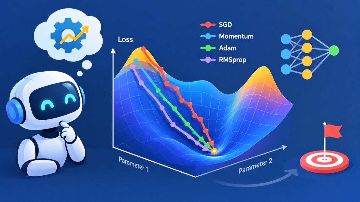
It’s difficult to overstate how popular gradient descent really is, and it’s used across the board even up to complex neural net architectures (backpropagation is basically gradient descent implemented on a network). There are other types of optimizers based on gradient descent that are used though, and here are a few of them:
Adagrad
Adagrad adapts the learning rate specifically to individual features: that means that some of the weights in your dataset will have different learning rates than others. This works really well for sparse datasets where a lot of input examples are missing. Adagrad has a major issue though: the adaptive learning rate tends to get really small over time. Some other optimizers below seek to eliminate this problem.
RMSprop
RMSprop is a special version of Adagrad developed by Professor Geoffrey Hinton in his neural nets class. Instead of letting all of the gradients accumulate for momentum, it only accumulates gradients in a fixed window. RMSprop is similar to Adaprop, which is another optimizer that seeks to solve some of the issues that Adagrad leaves open.
Adam
Adam stands for adaptive moment estimation, and is another way of using past gradients to calculate current gradients. Adam also utilizes the concept of momentum by adding fractions of previous gradients to the current one. This optimizer has become pretty widespread, and is practically accepted for use in training neural nets.
It’s easy to get lost in the complexity of some of these new optimizers. Just remember that they all have the same goal: minimizing our loss function. Even the most complex ways of doing that are simple at their core.